DATA146

Project 5 Part I

Question 1

First, we need to import the file persons.csv by using the command df = pd.read_csv("persons.csv"). By using df.isnull().values.any(), I found out that there are NaNs that needed to be removed. Then I used df.dropna(inplace=True) to remove all the NaNs. Observing the data frame again, I noticed that the number of rows decreased from 47974 to 47891, which is not a significant drop, so it would not influence the data too much. Also, we need to change the type of some features. By using display(df.dtypes), I found out that the “age” and “edu” features are both in the type of float. Thus, I utilized the astype method to convert them into int by using the command df["age"]=df["age"].astype(int) and the same thing for “edu.” Next, we need to assign the features to x and target to y. One thing to note here is that we would want to also drop the feature of wealthI along with wealthC when assigning x.

df = pd.read_csv("persons.csv")

df.dropna(inplace=True)
df.isnull().values.any()

df["age"]=df["age"].astype(int)
df["edu"]=df["edu"].astype(int)

X = df.drop(["wealthC", "wealthI"],axis=1)
y = df.wealthC

Question 2

Using linear regression without standardization, I produced a training MSE of 0.4428243604530385 and a testing MSE of 0.4437436624209024. The training R squared value is 0.7358226925730342 and the testing value is 0.7351080478691341. The coefficient the linear regression model without standardization is:

[ 3.01812923e-02,  1.07882853e-02, -5.57603897e-04,  8.37880684e-02,
  4.04701739e-02,  6.37198352e-02, -1.40023112e-01,  9.99896825e-02,
  1.85515805e-01, -2.49517259e-01, -2.47122665e-01, -7.30324831e-02,
  3.09612080e-01, -1.29375995e-01,  3.53607318e-01,  2.33225714e-01,
  -1.34364084e-01, -1.92558301e-01, -1.20146711e-01,  3.59279100e-02,
  1.46004504e-01, -1.81932414e-01,  1.05944573e-01,  4.00186663e-01,
  1.72822325e-01,  2.29943453e-02,  1.03043774e-01, -1.15888783e-01,
 -2.18966624e-01, -2.90949455e-01, -3.83672661e-01, -3.84737293e-01,
  3.07519898e-01,  2.55401258e-02,  2.56163113e-01,  3.95033383e-01,
  3.60442298e-01,  1.90435535e-01,  3.86891012e-01,  1.53405264e-01,
 -2.09042764e-02,  5.43122461e-02, -1.27172669e-01, -5.40268677e-01,
 -5.63637093e-01, -1.58355761e-01, -1.08923385e-01, -2.12578757e-02,
 -3.26132080e-01,  3.26132080e-01, -6.44297719e-02,  6.44297719e-02,
 -2.76390443e-01,  4.32693258e-01,  6.03439291e-02,  4.07576086e-01,
 -6.37787977e-01,  1.35651470e-02, -2.47897601e-01,  2.47897601e-01]

After standardization, the values of MSE and R squared are approximately the same with those generated by the linear regression model without standardization. The training MSE is 0.442836447539973 and the testing MSE is 0.44375982938707115. The training R squared is 0.735806256433555 and the testing value is 0.7349959689721618. We can see a slight drop in the testing R squared value and an increase in testing MSE after standardization, but it’s only minimal. However, we can see more changes in the coefficients of the standardized model. The coefficient of the standardized linear regression model is:

[ 1.12548658e-01  5.24358116e-03 -1.08884589e-02  6.92579735e-02
  7.36951509e+10  8.66257201e+10  7.69209583e+10  7.91372426e+10
  8.45473781e+10  7.89854838e+10  7.88333540e+10  8.76583681e+10
  8.66134726e+10  8.54267349e+10  1.16140874e+11  1.01070442e+11
  7.65053798e+10  7.51091695e+10  8.19133567e+10  4.80000747e+10
  7.26531241e+10  7.87003037e+10 -6.56609287e+09 -6.60161265e+09
 -1.20447035e+10 -1.40140921e+10 -7.23238899e+10 -3.56557715e+10
 -1.50138208e+10 -2.23537221e+10 -6.34833466e+10 -4.69533271e+09
 -7.80211026e+09 -1.23673099e+10 -1.59629508e+10  5.30991560e+10
  2.31813714e+11  8.95044996e+10  4.32553262e+10  1.67206073e+10
  3.49539754e+11  2.11161816e+11  2.27988135e+11  4.41825617e+11
  1.81354767e+10  2.62747629e+10  1.66594092e+11  3.43909538e+10
 -2.42890031e+11 -2.42890031e+11  1.82248582e+10  1.82248582e+10
  1.21238081e+10  5.65381739e+09  1.10197079e+10  2.38345511e+11
  2.39952072e+11  3.49669495e+10 -4.32651302e+10 -4.32651302e+10]

From the results we produced above, we can tell that standardizing the features actually made coefficients change quite a lot while the MSE and R squared values barely changed. Thus, we can conclude that standardization impacts the coefficients more than it does on MSE and R squared.

Question 3

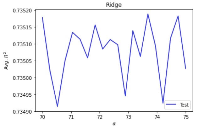
Using the ridge regression, I set the range from 70 to 75 and the number of folds to 20. This produced an optimal alpha value of 73.6842105263158, a training score of 0.7358356156922558, and a testing score of 0.7351887388305168. Compared with the scores produced by the linear regression model, the results produced by the ridge regression have seen a slight improvement, but the improvement only shows after the 4th decimal place.

Question 4

Using the lasso regression, I set the range from 0 to 0.5 and the number of folds to 20 to keep it consistent with the other models. This produced an optimal alpha value of 0, a training score of 0.7358355537426604, and a testing score of 0.7351336602401048. I was unsure at first if yielding a 0 as the optimal alpha value is normal. However, running the model for multiple times, I was still getting the same value of 0. Compared to the results produced by the linear regression model, we can also see an improvement, but it only appears after the 4th decimal place. In comparison with the ridge regression model, both the training and testing scores produced by the lasso regression model have both declined a little bit, so for the target variable wealthC, the ridge regression model has the best performance.

Question 5

With wealthI as the target, the linear regression model without standardization produced a MSE as high as 1750276834.930475, a training R squared value of 0.8258275464590519, and a testing R squared value of 0.8252769318036336. And the coefficient for the model is:

[ 2.31986195e+03,  1.08192000e+03, -5.08892487e+01,  6.53283809e+03,
  3.17688859e+03,  4.03623951e+03, -9.96051610e+03,  1.12302854e+04,
  1.02336910e+04, -1.62924258e+04, -1.71918653e+04, -6.04206999e+03,
  2.08751277e+04, -9.31120042e+03,  2.41734580e+04,  1.34930387e+04,
 -6.80151578e+03, -1.25300357e+04, -9.08909982e+03,  5.48192929e+03,
  7.99367502e+03, -1.34756043e+04,  1.74439055e+04,  3.27144540e+04,
  5.76665872e+03,  3.89473708e+02,  2.46689944e+03, -1.29356339e+04,
 -1.29054696e+04, -2.77376917e+04, -2.95652191e+04, -2.65078796e+04,
  2.29944393e+04, -3.88963009e+03,  3.17656932e+04,  4.00606955e+04,
  3.66535576e+04,  9.64026616e+03,  4.80974344e+04,  9.98177625e+03,
 -1.07028288e+04, -9.12002749e+03, -1.86232403e+04, -4.61832386e+04,
 -3.14138344e+04, -7.19146447e+03, -1.55796604e+04, -5.61943537e+03,
 -3.46563978e+04,  3.46563978e+04, -3.20570735e+04,  3.20570735e+04,
  1.51485651e+03,  5.89549456e+04,  2.36376276e+04,  9.41611219e+03,
 -6.81569745e+04, -2.53665673e+04, -2.24372689e+04,  2.24372689e+04]

After standardizing the linear regression model, the values of MSE and R squared barely changed. The training and testing MSE are 1750255416.6526966 and 1754915063.1109443 respectively. And the training and testing R squared values are 0.8258286888539557 and 0.8251401373199106. The coefficient of the linear regression model with standardization is:

[ 8.64993728e+03  5.31704713e+02 -1.00083919e+03  5.39975577e+03
  5.08584139e+15  5.97820436e+15  5.30846044e+15  5.46141040e+15
  5.83477406e+15  5.45093724e+15  5.44043848e+15  6.04946935e+15
  5.97735914e+15  5.89546013e+15  8.01510082e+15  6.97506186e+15
  5.27978059e+15  5.18342548e+15  5.65299528e+15  3.31257571e+15
  5.01392915e+15  5.43125643e+15 -4.53138456e+14 -4.55589743e+14
 -8.31227714e+14 -9.67138936e+14 -4.99120808e+15 -2.46067205e+15
 -1.03613210e+15 -1.54267253e+15 -4.38110551e+15 -3.24033768e+14
 -5.38438348e+14 -8.53491387e+14 -1.10163335e+15  3.66447293e+15
  1.59979017e+16  6.17687436e+15  2.98513166e+15  1.15392065e+15
  2.41223979e+16  1.45726753e+16  1.57338913e+16  3.04912193e+16
  1.25156346e+15  1.81327095e+15  1.14969726e+16  2.37338460e+15
 -1.67622992e+16 -1.67622992e+16  1.25773184e+15  1.25773184e+15
  8.36686869e+14  3.90180604e+14  7.60490828e+14  1.64486734e+16
  1.65595452e+16  2.41313515e+15 -2.98580826e+15 -2.98580826e+15]

From the above models using linear regression, we can see that the R squared value has increased in comparison with that of using wealthC, but the problem is that we now have extremely huge MSE which is not a positive sign for model prediction. Also, while the coefficients changed significantly, the values of MSE and R squared stay approximately the same.

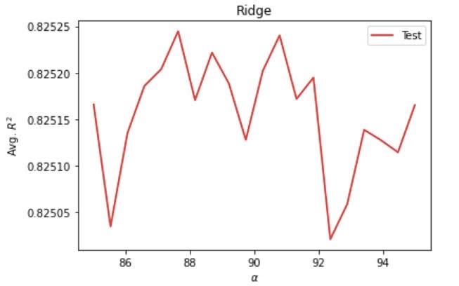
Running a ridge regression model, I set the range from 85 to 95 and the number of folds to 20. This produced an optimal alpha value of 87.15789473684211, a training score of 0.8258366475526164, and a testing score of 0.8253087200542343.

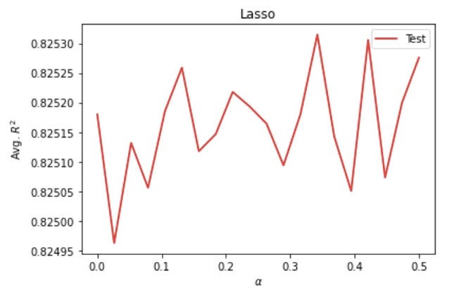
Running a lasso regression model, I set the range from 0 to 0.5 and the number of folds to 20. This produced an optimal alpha value of 0.3421052631578947, a training score of 0.8258367743818826, and a testing score of 0.825314711449513.

Question 6

Overall, there is much to take into consideration to identify the best model. In terms of R squared, all three kinds of models using wealthI have consistently higher values for training and testing scores than those using wealthC. This indicates that wealthI is a more correlated variable to the other variables in the persons.csv data set than wealthC, making it more suitable for predicting the wealth level for all people in the West African country. I had a concern regarding using wealthI though since it generates extremely large MSE, but right now I would assume R squared as a more important indicator than MSE when choosing the best model. Therefore, I think the models that produce the best results are the ridge and lasso regression models using wealthI since they generate about the same as well as the highest training and testing scores among all of the models for both wealthC and wealthI.

Below are the ridge and lasso regression models with wealthI as the target. From the graphs below, we can see that even the lowest R squared values in both models are higher than the maximum R squared values for the ridge regression model using wealthC.

Here is the ridge regression model using wealthC as the target. The reason why I only included the ridge regression model for wealthC here is because it is the best performing model among the three models using wealthC.